

Microsoft Excel is an extremely popular Office application among students, offices, researchers. It facilitates a plethora of options to create a huge table. You can create graphs, pie charts, trends of a particular business or scientific model and so on. The numbers of features are almost endless.
As we all know, MS Excel is often used as an efficient data analysis tool. We often work with huge data set, and to understand about the nature of the data, the trend, the variation, we have to perform data analysis on our data. Quick analysis enables you to perform many more formatting like color codes, greater than, less than, icon set, color scale, etc. There are provisions for various tables, pivot tables, charts, etc.
While perfoming mathematical analysis, over a large range of data, a user may need to find out the average of all the values of a column. The process is not as tedious as it seems. Students can use the Total Row option to find out the total value of any cells of a column, or all columns. By following the same method, you can find out the SUM, Count, Greatest, Least, IF, etc as well.
Steps To Find The Average Of A Particular Column In MS Excel?
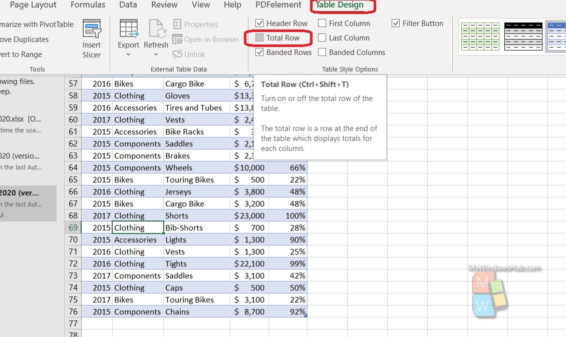
First tap in any cell of the table. Now go to Table Design. Check the box beside Total Row option.
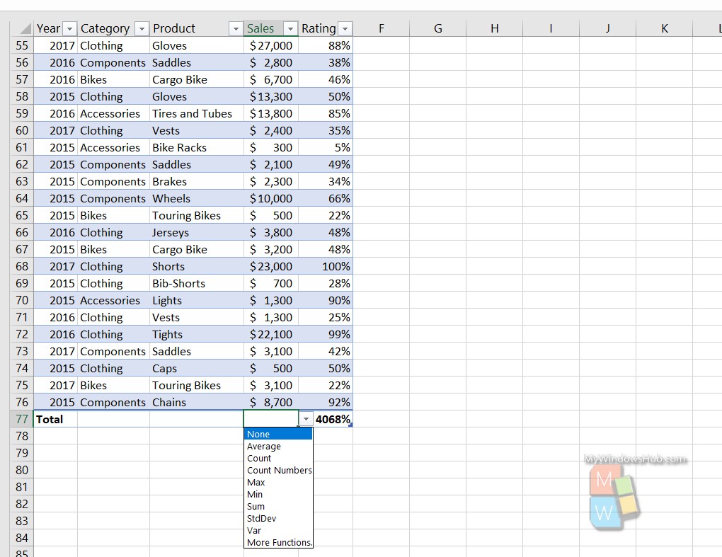
Next, click on any bottom row total cell. A dropdown arrow will appear along with the cell. Click on it and select the function, you want, for e.g. AVERAGE.
It’s done! You can select that cell and then expand towards right to apply the same functions on the other rows as well.