Microsoft Excel is an extremely popular Office application among students, offices, researchers. It facilitates a plethora of options to create a huge table. You can create graphs, pie charts, trends of a particular business or scientific model and so on. The numbers of features are almost endless.
If you are working with a large number of rows, with numerous elements on it, it is very obvious to get lost amid so many rows and columns. To identify each and every row, you can create Banded row look, with alternate colored bands on the rows, to create a better perception and visibility.
In this tutorial, I shall show you the simple way to create banded rows in MS Excel Worksheet.

Steps To Create Banded Rows In An MS Excel Worksheet
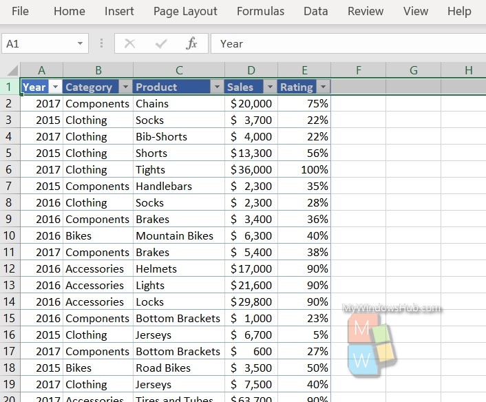
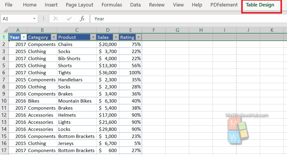
First, open the MS Excel worksheet and click on Table Design.

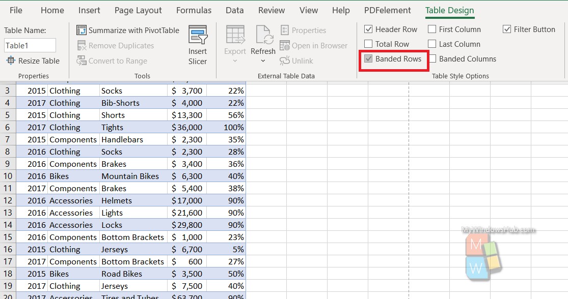
You will find an option called Banded Rows. Check the option to enable it.

That’s all!

